Postprocessing
[1]:
%matplotlib inline
%config InlineBackend.figure_format = 'retina'
%load_ext autoreload
%load_ext line_profiler
%load_ext snakeviz
%autoreload 2

import numpy as np
import matplotlib
import matplotlib.pyplot as plt
import corner

import pickle

import enterprise
from enterprise.pulsar import Pulsar
import enterprise.signals.parameter as parameter
from enterprise.signals import utils
from enterprise.signals import signal_base
from enterprise.signals import selections
from enterprise.signals.selections import Selection
from enterprise.signals import white_signals
from enterprise.signals import gp_signals
from enterprise.signals import deterministic_signals
import enterprise.constants as const

from enterprise_extensions import deterministic

from scipy.stats import norm

import libstempo as T2
import libstempo.toasim as LT
import libstempo.plot as LP

import glob
import json
import h5py
import healpy as hp
import scipy.constants as sc
import emcee

from numba.typed import List
WARNING: AstropyDeprecationWarning: The private astropy._erfa module has been made into its own package, pyerfa, which is a dependency of astropy and can be imported directly using "import erfa" [astropy._erfa]
[ ]:
#load psr pickles

#make sure this points to the same pickled pulsars we used for the MCMC
data_pkl = '../data/quickCW_test_psrs.pkl'

#with open('nanograv_11yr_psrs_old.pkl', 'rb') as psr_pkl:
with open(data_pkl, 'rb') as psr_pkl:
    psrs = pickle.load(psr_pkl)

print(len(psrs))
[2]:
#load psr names only if we want to save RAM
class psr_name:
    def __init__(self, name):
        self.name = name

psrListFile = "../data/quickCW_test_psrlist.txt"

psrs = []
with open(psrListFile, 'r') as fff:
    for line in fff:
        psrname = line.strip()
        #print(psrname)
        psrs.append(psr_name(psrname))

print(len(psrs))
for i,psr in enumerate(psrs):
    print(str(i) + ": " + psr.name)
67
0: B1855+09
1: B1937+21
2: B1953+29
3: J0023+0923
4: J0030+0451
5: J0340+4130
6: J0406+3039
7: J0437-4715
8: J0509+0856
9: J0557+1551
10: J0605+3757
11: J0610-2100
12: J0613-0200
13: J0636+5128
14: J0645+5158
15: J0709+0458
16: J0740+6620
17: J0931-1902
18: J1012+5307
19: J1012-4235
20: J1022+1001
21: J1024-0719
22: J1125+7819
23: J1312+0051
24: J1453+1902
25: J1455-3330
26: J1600-3053
27: J1614-2230
28: J1630+3734
29: J1640+2224
30: J1643-1224
31: J1705-1903
32: J1713+0747
33: J1719-1438
34: J1730-2304
35: J1738+0333
36: J1741+1351
37: J1744-1134
38: J1745+1017
39: J1747-4036
40: J1751-2857
41: J1802-2124
42: J1811-2405
43: J1832-0836
44: J1843-1113
45: J1853+1303
46: J1903+0327
47: J1909-3744
48: J1910+1256
49: J1911+1347
50: J1918-0642
51: J1923+2515
52: J1944+0907
53: J1946+3417
54: J2010-1323
55: J2017+0603
56: J2033+1734
57: J2043+1711
58: J2124-3358
59: J2145-0750
60: J2214+3000
61: J2229+2643
62: J2234+0611
63: J2234+0944
64: J2302+4442
65: J2317+1439
66: J2322+2057
Load run + general diagnostics
[3]:
#load results from HDF5 file

hdf_file = "../results/quickCW_test.h5"

with h5py.File(hdf_file, 'r') as f:
    print(list(f.keys()))
    samples_cold = f['samples_cold'][0,::10,:]
    print(f['samples_cold'].dtype)
    #samples = f['samples_cold'][...]
    #log_likelihood = f['log_likelihood'][:,::10]
    print(f['log_likelihood'].dtype)
    log_likelihood = f['log_likelihood'][...]
    par_names = [x.decode('UTF-8') for x in list(f['par_names'])]
    acc_fraction = f['acc_fraction'][...]
    fisher_diag = f['fisher_diag'][...]

#print(acc_fraction)
#print(acc_fraction[:,:])
#print(samples.shape)
#samples_cold = np.copy(samples[0,:,::])
print(samples_cold.shape)
#print(par_names)
['T-ladder', 'acc_fraction', 'fisher_diag', 'log_likelihood', 'par_names', 'samples_cold', 'samples_freq']
float32
float64
(1000000, 278)
[ ]:
#Plot acceptance fraction for different kinds of steps as a function of PT chain - good for checking is run is okay

plt.figure(0)
plt.plot(acc_fraction[-2,:], color='xkcd:grey', ls='-', marker='.', label="PT")
plt.plot(acc_fraction[-1,:], color='xkcd:blue', ls='-', marker='.', label="Projection parameters")
plt.ylim(0,1)
plt.legend(bbox_to_anchor=(1,1), loc="upper left")
plt.xlabel("PT chain number")
plt.ylabel("Acceptance rate")


plt.figure(1)
plt.plot(acc_fraction[1,:], color='xkcd:green', ls='-', marker='.', label="PSR distance (prior draw)")
plt.plot(acc_fraction[3,:], color='xkcd:light green', ls='-', marker='.', label="PSR distance (DE)")
plt.plot(acc_fraction[5,:], color='xkcd:olive', ls='-', marker='.', label="PSR distance (fisher)")
plt.ylim(0,1)
plt.legend(bbox_to_anchor=(1,1), loc="upper left")
plt.xlabel("PT chain number")
plt.ylabel("Acceptance rate")


plt.figure(2)
plt.plot(acc_fraction[7,:], color='xkcd:dark red', ls='-', marker='.', label="RN (empirical distribution)")
plt.plot(acc_fraction[9,:], color='xkcd:red', ls='-', marker='.', label="RN (DE)")
plt.plot(acc_fraction[11,:], color='xkcd:pink', ls='-', marker='.', label="RN (fisher)")
plt.ylim(0,1)
plt.legend(bbox_to_anchor=(1,1), loc="upper left")
plt.xlabel("PT chain number")
plt.ylabel("Acceptance rate")


plt.figure(3)
plt.plot(acc_fraction[13,:], color='xkcd:purple', ls='-', marker='.', label="GWB (prior draw)")
plt.plot(acc_fraction[15,:], color='xkcd:dark purple', ls='-', marker='.', label="GWB (DE)")
plt.plot(acc_fraction[17,:], color='xkcd:light purple', ls='-', marker='.', label="GWB (fisher)")
plt.ylim(0,1)
plt.legend(bbox_to_anchor=(1,1), loc="upper left")
plt.xlabel("PT chain number")
plt.ylabel("Acceptance rate")

plt.figure(4)
plt.plot(acc_fraction[19,:], color='xkcd:blue', ls='-', marker='.', label="Common parameters (prior draw)")
plt.plot(acc_fraction[21,:], color='xkcd:dark blue', ls='-', marker='.', label="Common parameters (DE)")
plt.plot(acc_fraction[23,:], color='xkcd:aqua', ls='-', marker='.', label="Common parameters (fisher)")
plt.ylim(0,1)
plt.legend(bbox_to_anchor=(1,1), loc="upper left")
plt.xlabel("PT chain number")
plt.ylabel("Acceptance rate")

plt.figure(5)
plt.plot(acc_fraction[25,:], color='xkcd:orange', ls='-', marker='.', label="All (prior draw)")
plt.plot(acc_fraction[27,:], color='xkcd:dark orange', ls='-', marker='.', label="All (DE)")
plt.plot(acc_fraction[29,:], color='xkcd:light orange', ls='-', marker='.', label="All (fisher)")
plt.ylim(0,1)
plt.legend(bbox_to_anchor=(1,1), loc="upper left")
plt.xlabel("PT chain number")
plt.ylabel("Acceptance rate")
[ ]:
#plot the trace of the likelihood values to see if its sensible
for j in range(1):
    plt.plot(log_likelihood[j,10::1], label=str(j))

plt.legend()
[ ]:
#also plot the histogram of likelihoods
_ = plt.hist(log_likelihood[0,10_000::1], density=True, bins=100)
plt.yscale('log')
#plt.xlim(3_302_770, 3_302_860)
plt.ylim(1e-7,1e-1)
[ ]:
#set up dictionary with true values of parameters
#set it to nan where not known

KPC2S = sc.parsec / sc.c * 1e3
SOLAR2S = sc.G / sc.c ** 3 * 1.98855e30

xxx = {"0_cos_gwtheta":np.nan,
       "0_cos_inc":np.nan,
       "0_gwphi":np.nan,
       "0_log10_fgw":np.nan,
       "0_log10_h":np.nan,
       "0_log10_mc":np.nan,
       "0_phase0":np.nan,
       "0_psi":np.nan}

singwtheta = np.sin(np.arccos(xxx['0_cos_gwtheta']))
cosgwtheta = xxx['0_cos_gwtheta']
singwphi = np.sin(xxx["0_gwphi"])
cosgwphi = np.cos(xxx["0_gwphi"])
omhat = np.array([-singwtheta * cosgwphi, -singwtheta * singwphi, -cosgwtheta])

with open('../data/quickCW_noisedict.json', 'r') as fp:
        noisedict = json.load(fp)

for j in range(len(psrs)):
    xxx[psrs[j].name+"_red_noise_gamma"] = noisedict[psrs[j].name+"_red_noise_gamma"]
    xxx[psrs[j].name+"_red_noise_log10_A"] = noisedict[psrs[j].name+"_red_noise_log10_A"]
    xxx[psrs[j].name+"_cw0_p_dist"] = 0.0

    #ptheta = psrs[j].theta
    #pphi = psrs[j].phi
    #
    #phat = np.array([np.sin(ptheta) * np.cos(pphi), np.sin(ptheta) * np.sin(pphi), np.cos(ptheta)])
    #cosMu = -np.dot(omhat, phat)
    #
    #pphase = (1 + 256/5 * (10**xxx['0_log10_mc']*SOLAR2S)**(5/3) * (np.pi * 10**xxx['0_log10_fgw'])**(8/3)
    #          * psrs[j].pdist[0]*KPC2S*(1-cosMu)) ** (5/8) - 1
    #pphase /= 32 * (10**xxx['0_log10_mc']*SOLAR2S)**(5/3) * (np.pi * 10**xxx['0_log10_fgw'])**(5/3)
    #
    #xxx[psrs[j].name+"_cw0_p_phase"] = -pphase%(2*np.pi)
    xxx[psrs[j].name+"_cw0_p_phase"] = np.nan

xxx['gwb_gamma'] = np.nan
xxx['gwb_log10_A'] = np.nan

print(xxx)
Parameter traces and corner plots
[ ]:
#get autocorrelation lengths
#burnin = 0
burnin = 50_000
thin = 10

ccs = np.zeros(len(par_names))

for i, par in enumerate(par_names):
    ccs[i] = emcee.autocorr.integrated_time(samples_cold[burnin::thin,i], c=10, quiet=True)
    print(par, str(ccs[i]))
[ ]:
_ = plt.hist(np.log10(ccs), bins=100)
print(samples_cold.shape[0]-burnin)
sort_idx = np.argsort(ccs)
for idx in sort_idx[:-30:-1]:
    print(par_names[idx], str(ccs[idx]))
[ ]:
#plot trace of all parameters
for i, par in enumerate(par_names):
    plt.figure(i)
    plt.plot(samples_cold[::100,i], ls='', marker='.')
    plt.gca().axhline(xxx[par], ls='--')

    plt.title(str(i) + ": " + par)
[ ]:
#corner plot of parameters common to all pulsars
corner_mask = [0, 1, 2, 3, 4, 5, 6, 7]
par_keys = ["0_cos_gwtheta", "0_cos_inc", "0_gwphi", "0_log10_fgw",
          "0_log10_h", "0_log10_mc", "0_phase0", "0_psi"]
labels = [r"$\cos \theta$", r"$\cos \iota$", r"$\phi$", r"$\log_{10} f_{\rm GW}$",
          r"$\log_{10} A_{\rm e}$", r"$\log_{10} {\cal M}$", r"$\Phi_0$", r"$\psi$"]


#set ranges
ranges = [(-1,1), (-1,1), (0,2*np.pi), (np.log10(3.5e-9),-7), (-18,-11), (7,10), (0,2*np.pi), (0,np.pi) ]

#set burnin and thinning
burnin = 100
thin = 10

truth = [xxx[key] for key in par_keys]
fig = corner.corner(samples_cold[burnin::thin,corner_mask], labels=labels, #show_titles=True, quantiles=[0.16, 0.5, 0.84],
                    truths=truth, range=ranges, hist_kwargs={"density":True})

#plot priors over 1D posteriors
for i, ax in enumerate(fig.axes):
    if i==0 or i==(len(labels)+1): #cos inc and cos theta
        Xs = np.linspace(-1,1)
        ax.plot(Xs, Xs*0+1/2, color="xkcd:green")
    elif i==2*(len(labels)+1) or i==6*(len(labels)+1): #gwphi and phase0
        Xs = np.linspace(0,2*np.pi)
        ax.plot(Xs, Xs*0+1/(2*np.pi), color="xkcd:green")
    elif i==3*(len(labels)+1): #log10_fgw
        Xs = np.linspace(np.log10(3.5e-9), -7.0)
        ax.plot(Xs, Xs*0+1/(-7-np.log10(3.5e-9)), color="xkcd:green")
    elif i==4*(len(labels)+1): #log10_A
        Xs = np.linspace(-18, -11)
        ax.plot(Xs, Xs*0+1/7, color="xkcd:green")
    elif i==5*(len(labels)+1): #log10_M_ch
        Xs = np.linspace(7, 10)
        ax.plot(Xs, Xs*0+1/3, color="xkcd:green")
    elif i==7*(len(labels)+1): #psi
        Xs = np.linspace(0,np.pi)
        ax.plot(Xs, Xs*0+1/np.pi, color="xkcd:green")
[ ]:
#corner plots for pulsar specific parameters

for I, psr in enumerate(psrs[:]):
    plt.figure(I)
    print(psr.name)
    corner_mask = [8+I*4, 9+I*4, 10+I*4, 11+I*4]
    labels = ["{0}_cw0_p_dist".format(psr.name), "{0}_cw0_p_phase".format(psr.name),
              "{0}_red_noise_gamma".format(psr.name), "{0}_red_noise_log10_A".format(psr.name)]
    #ranges = [(-3,3), (0, 2*np.pi), 0.999, 0.999]
    ranges = [(-3,3), (0, np.pi), (0,7), (-20,-11)]

    burnin = 100
    thin = 10

    truth = [xxx[key] for key in labels]
    fig = corner.corner(samples_cold[burnin::thin,corner_mask], labels=labels,
                        truths=truth, range=ranges, hist_kwargs={"density":True})

    Xs = np.linspace(0,2*np.pi)
    Ys = np.linspace(-3.0,3.0)
    Zs = np.linspace(0.0,7.0)
    Qs = np.linspace(-20.0, -11.0)

    for i, ax in enumerate(fig.axes):
        if i%(len(labels)+1)==0:
            if i%(4*(len(labels)+1))==0: #psr distance
                ax.plot(Ys, norm.pdf(Ys), color="xkcd:green")
            elif i%(4*(len(labels)+1))==1*(len(labels)+1): #psr phase
                ax.plot(Xs, Xs*0+1/(2*np.pi), color="xkcd:green")
            elif i%(4*(len(labels)+1))==2*(len(labels)+1): #rn gamma
                ax.plot(Zs, Zs*0+1/7.0, color="xkcd:green")
            elif i%(4*(len(labels)+1))==3*(len(labels)+1): #rn log_10_A
                ax.plot(Qs, Qs*0+1/9.0, color="xkcd:green")
        #print(ax.set_xlabel(i))
[ ]:
#gwb
corner_mask = [-2, -1]
labels = ["gwb_gamma", "gwb_log10_A"]
#ranges = [0.999, ]*8
ranges = [(0,7), (-20,-11)]

#burnin = 0
#burnin = 50_000
burnin = 100_000
thin = 10

truth = [xxx[key] for key in labels]
fig = corner.corner(samples_cold[burnin::thin,corner_mask], labels=labels,
                    truths=truth, range=ranges, hist_kwargs={"density":True})
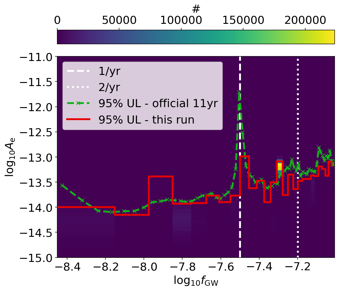
UL vs. frequency
[4]:
official_11yr_skyavg = np.loadtxt("../data/11yr_ul_skyavg_DE436.txt")
[11]:
%%time
plt.rcParams.update({'font.size': 18})

#burnin = 100_000
burnin = 50_000
thin=1
#thin = 10*int(np.max([ccs[3],ccs[4]]))
print(thin)

log10_fgws = samples_cold[burnin::thin,3]
log10_hs = samples_cold[burnin::thin,4]
print(log10_fgws.size)


"""f_bincenters = official_11yr_skyavg[1:67,0]
#f_bincenters = official_11yr_skyavg[1:8,0]
print(f_bincenters)
f_bins = []
for i in range(f_bincenters.shape[0]-1):
    f_bins.append(f_bincenters[i]-(f_bincenters[i+1]-f_bincenters[i])/2)
f_bins.append(f_bincenters[-1]-(f_bincenters[-1]-f_bincenters[-2])/2)
f_bins.append(f_bincenters[-1]+(f_bincenters[-1]-f_bincenters[-2])/2)
print(f_bins)"""

f_min = 10**np.min(samples_cold[::10,3])
f_max = 10**np.max(samples_cold[::10,3])
print(f_min, f_max)
#f_bins = np.linspace(f_min, f_max, int(f_max/f_min))
f_bins = np.arange(1,int(f_max/f_min)+1)*f_min
print(f_bins)

f_bincenters = []
for i in range(f_bins.size-1):
    f_bincenters.append((f_bins[i+1]+f_bins[i])/2)
print(f_bincenters)

log10_h_bins = np.linspace(-18,-11,100)

plt.figure(figsize=(8,7))
#h, xedges, yedges, _ = plt.hist2d(log10_fgws, log10_hs, bins=50, range=[[np.log10(3.5e-9),-7],[-18,-11]])
#h, xedges, yedges, _ = plt.hist2d(log10_fgws, log10_hs, bins=100, range=[[np.log10(3.5e-9),-7],[-15.5,-11]],
#                                  weights=log10_fgws*0+1/60.0)
h, xedges, yedges, _ = plt.hist2d(log10_fgws, log10_hs, bins=[np.log10(f_bins), log10_h_bins])

#make bin centers
bincenters = []
for i in range(xedges.size-1):
    bincenters.append((xedges[i+1]+xedges[i])/2)
bincenters = np.array(bincenters)

#print(xedges)
#print(bincenters)

freq_idx = np.digitize(log10_fgws, xedges)
#plt.scatter(log10_fgws[np.where(freq_idx==1)], log10_hs[np.where(freq_idx==1)])

N_bootstrap = 1000
#N_resample = 100

UL_freq = np.zeros(bincenters.size)
#UL_freq_reweight = np.zeros(bincenters.size)
#UL_freq_reweight_low = np.zeros(bincenters.size)
#UL_freq_reweight_high = np.zeros(bincenters.size)
UL_freq_error = np.zeros(bincenters.size)
for i in range(bincenters.size):
    print('---')
    print(i)
    hs = 10**log10_hs[np.where(freq_idx==i+1)]
    if hs.size==0:
        UL_freq[i] = 0.0
        continue

    UL_freq[i] = np.percentile(hs, 95)

    N_inbin = hs.shape[0]
    N_resample = int(N_inbin)

    print(N_inbin)

    #N_batch = int(N_inbin**(1/5))
    N_batch = 10
    if N_inbin<10*N_batch:
        N_batch=1
    print(N_batch)

    hs_batches = []
    for K in range(N_batch):
        hs_batches.append(hs[K*int(N_inbin/N_batch):(K+1)*int(N_inbin/N_batch)])

    ULs = np.zeros(N_bootstrap)
    for k in range(N_bootstrap):
        IDXS = np.random.choice(N_batch, size=N_batch, replace=True)
        hs_shuffle = np.block([hs_batches[J] for J in IDXS])
        ULs[k] = np.percentile(hs_shuffle, 95)

    UL_freq_error[i] = np.std(ULs)


plt.gca().axvline(x=-np.log10(3600*24*365.24), ls='--', lw=3, color='white', label='1/yr')
plt.gca().axvline(x=-np.log10(3600*24*365.24*0.5), ls=':', lw=3, color='white', label='2/yr')
#plt.plot(bincenters, UL_freq, ls='-', lw=3, marker='.', color="xkcd:red", label="95% UL")
#plt.errorbar(bincenters, np.log10(UL_freq), ls='-', lw=3, marker='x', color="xkcd:red",
#             label="95% UL - this run - old", alpha=0.3)
plt.errorbar(xedges[:-1], np.log10(UL_freq), ls='-', lw=3, color="xkcd:red",
             drawstyle='steps-post', label="95% UL - this run")
#plt.fill_between(bincenters, UL_freq_reweight_low, UL_freq_reweight_high,
#                 color="xkcd:red", alpha=0.3, label="95% UL")
plt.plot(np.log10(official_11yr_skyavg[1:67,0]), np.log10(official_11yr_skyavg[1:67,1]),
         ls='--', lw=3, marker='x', color="xkcd:green", label="95% UL - official 11yr")
#plt.plot(np.log10(official_11yr_skyavg[:,0]), np.log10(official_11yr_skyavg[:,2]),
#         ls='--', lw=3, marker='.', color="xkcd:purple", label="95% UL - official2")
plt.ylim(-15,-11)
#plt.xlim(-8.75, -7.0)
plt.xlabel(r"$\log_{10} f_{\rm GW}$")
plt.ylabel(r"$\log_{10} A_{\rm e}$")

cbar = plt.colorbar(location='top')
cbar.set_label('#')

plt.legend(loc=2)

plt.tight_layout()  # otherwise the right y-label is slightly clipped
#plt.savefig("Figs/UL_vs_freq.png", dpi=300)
#plt.savefig("Figs/UL_vs_freq_new_seed.png", dpi=300)
1
950000
3.5255192563008488e-09 9.911633809173201e-08
[3.52551926e-09 7.05103851e-09 1.05765578e-08 1.41020770e-08
 1.76275963e-08 2.11531155e-08 2.46786348e-08 2.82041541e-08
 3.17296733e-08 3.52551926e-08 3.87807118e-08 4.23062311e-08
 4.58317503e-08 4.93572696e-08 5.28827888e-08 5.64083081e-08
 5.99338274e-08 6.34593466e-08 6.69848659e-08 7.05103851e-08
 7.40359044e-08 7.75614236e-08 8.10869429e-08 8.46124622e-08
 8.81379814e-08 9.16635007e-08 9.51890199e-08 9.87145392e-08]
[5.288278884451273e-09, 8.813798140752122e-09, 1.2339317397052971e-08, 1.586483665335382e-08, 1.939035590965467e-08, 2.2915875165955517e-08, 2.6441394422256365e-08, 2.9966913678557216e-08, 3.349243293485806e-08, 3.701795219115892e-08, 4.054347144745976e-08, 4.4068990703760606e-08, 4.759450996006146e-08, 5.112002921636231e-08, 5.464554847266315e-08, 5.817106772896401e-08, 6.169658698526485e-08, 6.522210624156571e-08, 6.874762549786655e-08, 7.22731447541674e-08, 7.579866401046824e-08, 7.93241832667691e-08, 8.284970252306995e-08, 8.63752217793708e-08, 8.990074103567165e-08, 9.342626029197249e-08, 9.695177954827334e-08]
---
0
40751
10
---
1
7970
10
---
2
11487
10
---
3
81594
10
---
4
14225
10
---
5
1534
10
---
6
276
10
---
7
11993
10
---
8
8475
10
---
9
466
10
---
10
930
10
---
11
2605
10
---
12
14944
10
---
13
658091
10
---
14
228
10
---
15
2975
10
---
16
2885
10
---
17
1928
10
---
18
7889
10
---
19
14442
10
---
20
41034
10
---
21
545
10
---
22
917
10
---
23
1013
10
---
24
5305
10
---
25
14944
10
---
26
485
10
CPU times: user 12.8 s, sys: 92.8 ms, total: 12.9 s
Wall time: 12.7 s
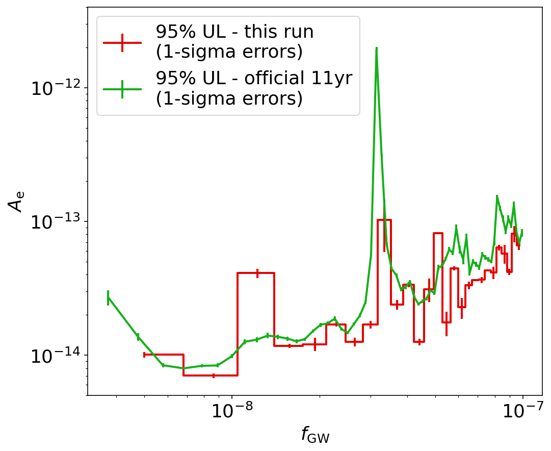
[18]:
plt.figure(figsize=(8,7))

plt.errorbar(10**bincenters, UL_freq, yerr=UL_freq_error,
             ls='', lw=2, marker='.', alpha=0., color="xkcd:red")

plt.errorbar(10**xedges[:-1], UL_freq, drawstyle='steps-post',
             ls='-', lw=2, marker='', alpha=1.0, color="xkcd:red", label="95% UL - this run\n(1-sigma errors)")

plt.errorbar(official_11yr_skyavg[1:67,0], official_11yr_skyavg[1:67,1],
             yerr=official_11yr_skyavg[1:67,2],
             ls='-', lw=2, marker='', color="xkcd:green", label="95% UL - official 11yr\n(1-sigma errors)")

plt.xscale('log')
plt.yscale('log')
plt.ylim(5e-15,4e-12)
plt.xlabel(r"$f_{\rm GW}$")
plt.ylabel(r"$A_{\rm e}$")

plt.legend(loc=2)
[18]:
<matplotlib.legend.Legend at 0x7f2f733ddc10>
[ ]:
[ ]: